
Updated for JKSSB JE Civil 2025
Category: Fluid Mechanics | Civil Engineering
📘 Introduction
In fluid mechanics, understanding the nature of flow is essential for analyzing and designing hydraulic structures like pipes, culverts, irrigation channels, and sewage systems. The two primary types of flow are:
- Laminar Flow: Smooth, orderly movement of fluid particles in layers.
- Turbulent Flow: Chaotic, random fluid motion with significant mixing and energy loss.
For JKSSB Civil Engineering aspirants, questions from this topic often appear in both theoretical and numerical form, especially related to Reynolds Number, head loss, and pipe flow design.
🔍 What is Laminar Flow?
Laminar flow is a type of fluid motion characterized by smooth, orderly, and parallel layers of fluid particles that move without disruption between the layers. In this flow regime, each particle of the fluid follows a well-defined path or streamline, and there is no mixing or cross-flow between adjacent layers. The flow velocity at any point remains constant over time, and the movement is steady and predictable.
Laminar flow typically occurs at low velocities and in fluids with high viscosity, where viscous forces dominate over inertial forces. Because of this dominance of viscous forces, the fluid particles move in a highly organized manner, allowing the flow to remain stable and laminar.
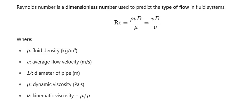
Mathematically, laminar flow is identified when the Reynolds number (Re) is less than approximately 2000. Reynolds number is a dimensionless parameter that represents the ratio of inertial forces to viscous forces in a fluid flow.
In practical terms, laminar flow is observed in systems such as the slow flow of syrup in a narrow pipe, blood flow in small capillaries, or oil moving through thin tubes.
Key points to remember:
- Fluid particles move in parallel layers or streamlines.
- There is no turbulence or mixing between layers.
- Flow velocity is steady and predictable.
- Dominated by viscous forces.
- Occurs at low Reynolds number (Re < 2000).
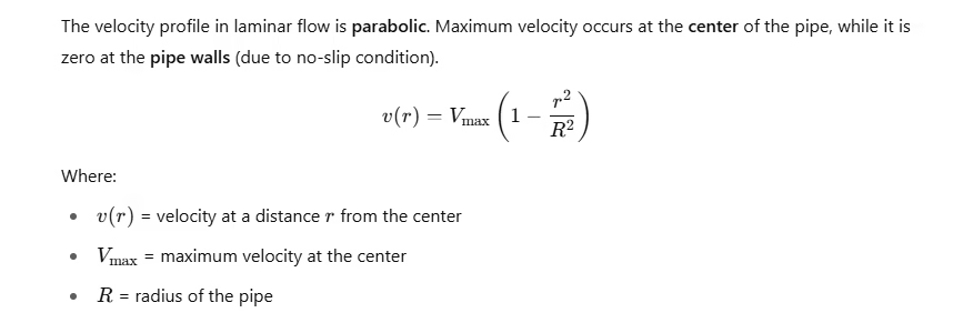
- Velocity profile is parabolic across the pipe cross-section.
Examples of Laminar Flow
- Flow of oil or glycerin through narrow pipes
Due to their high viscosity and low velocity, these fluids move smoothly in parallel layers without mixing. - Blood flow in small capillaries and arterioles
In tiny blood vessels, the flow velocity is low, resulting in laminar flow which is essential for efficient nutrient transport. - Flow of syrup or honey in thin tubes
These viscous fluids flow steadily in layers without turbulence. - Groundwater flow through soil or porous media
Movement of water underground through soil pores is slow and orderly, commonly modeled as laminar flow. - Flow inside viscometers
Devices that measure viscosity rely on laminar flow conditions to ensure accuracy. - Airflow over smooth surfaces at low speeds
At very low velocities, airflow close to surfaces can be laminar before becoming turbulent at higher speeds.
📐 Velocity Profile:
🌪️ What is Turbulent Flow?
Turbulent flow is a type of fluid motion characterized by irregular, chaotic, and random fluctuations in velocity and pressure. Unlike laminar flow, where fluid particles move smoothly in parallel layers, turbulent flow involves rapid mixing of fluid particles across the flow path. This mixing creates swirling vortices and eddies of various sizes, resulting in complex and unpredictable movement.
Turbulent flow occurs when the inertial forces in the fluid dominate over the viscous forces, which typically happens at high flow velocities, larger pipe diameters, or fluids with low viscosity. This leads to continuous changes in the magnitude and direction of the velocity at any point within the fluid.
The onset of turbulence is commonly predicted using the Reynolds number (Re), a dimensionless quantity representing the ratio of inertial to viscous forces. When the Reynolds number exceeds approximately 4000, the flow is generally turbulent.
Turbulent flow is associated with higher energy losses due to friction and eddy formation, which are significant factors in hydraulic design. The velocity profile in turbulent flow is relatively flatter compared to laminar flow, indicating more uniform velocity across the pipe’s cross-section except near the walls where a thin boundary layer exists.
Key points to remember:
Velocity profile is flatter than laminar flow.
Fluid motion is irregular, chaotic, and contains vortices.
Velocity changes continuously with time and position.
Dominated by inertial forces.
Occurs at high Reynolds number (Re > 4000).
Results in high energy loss due to friction and eddies.
Examples of Turbulent Flow
- Water flow in large rivers and canals
The velocity and irregularities in natural waterways cause chaotic and swirling fluid motion. - Flow of water through large-diameter pipes
High velocity and pipe size create turbulent conditions, common in municipal water supply systems. - Airflow over airplane wings and vehicles at high speed
At higher speeds, air becomes turbulent, causing fluctuations in pressure and drag. - Mixing of fluids in industrial processes
Rapid stirring or flow through mixers generates turbulence to enhance mixing efficiency. - Smoke rising from a chimney
The chaotic, swirling motion of smoke plumes is a classic example of turbulent flow. - Stormy ocean waves and waterfall flows
Natural phenomena where fluid motion is highly irregular and turbulent.
📐 Velocity Profile:
Velocity profile is flatter than in laminar flow, especially in the central region of the pipe. A thin boundary layer near the pipe wall still shows lower velocity.
📊 Difference Between Laminar and Turbulent Flow
| Property | Laminar Flow | Turbulent Flow |
|---|---|---|
| Flow Pattern | Smooth and layered | Irregular and chaotic |
| Reynolds Number | < 2000 | > 4000 |
| Dominant Forces | Viscous | Inertial |
| Velocity Profile | Parabolic | Flatter, more uniform |
| Energy Loss | Low | High |
| Mixing | Absent | Present |
| Application Examples | Syringes, Oil Flow in capillaries | Water supply pipes, rivers |
| Friction Factor | Inversely proportional to Re | Complex function of Re |
| Predictability | High | Low (random fluctuations) |
🔁 Transition Flow – Intermediate Zone
When Reynolds number is between 2000 and 4000, the flow is called transitional. In this range, the flow may alternate between laminar and turbulent, depending on factors like:
- Pipe roughness
- Flow disturbances
- Entrance effects
📍 Practical Implication:
Engineers avoid designing systems in this range due to unpredictability and instability of flow.
📏 Reynolds Number (Re)
🔢 Flow Classification:
| Reynolds Number (Re) | Type of Flow |
|---|---|
| Re < 2000 | Laminar |
| 2000 ≤ Re ≤ 4000 | Transition |
| Re > 4000 | Turbulent |
🧪 Practical Applications in Civil Engineering
Laminar Flow:
- Used in viscometer calibration
- Flow of highly viscous fluids like oil or glycerin
- Groundwater flow in aquifers (Darcy’s Law applicable)
Turbulent Flow:
- Water supply pipelines
- Drainage and sewer systems
- River and open channel flow
- Hydraulic turbines and spillways
Design Consideration:
- In laminar flow, head loss (hₗ) is directly proportional to velocity.
- In turbulent flow, head loss is approximately proportional to velocity².
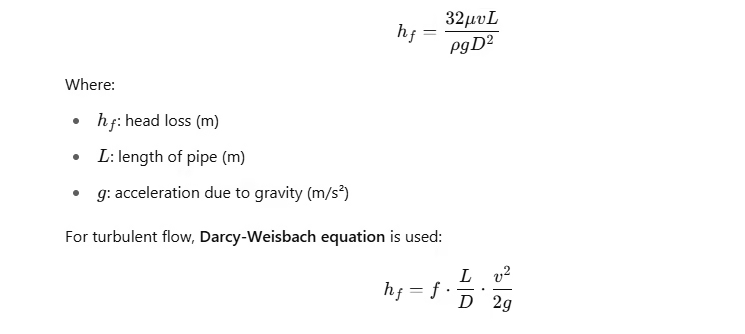
📉 Head Loss Formula (Hagen–Poiseuille’s Law – Laminar)
📌 JKSSB Civil Exam Relevance
JKSSB often asks:
- Conceptual MCQs on flow types
- Problems based on Reynolds number
- Velocity profile and friction loss
- Applications in hydraulic structures
📌 PYQ Example (JKSSB JE 2022):
Q: The flow is said to be laminar if Reynolds number is:
a) < 1000
b) < 2000
c) > 4000
d) Between 2000 and 4000
✔️ Correct Answer: b) < 2000
🎯 Memory Tricks
- LAMINAR → “LAyers Move In Neat And Regular lines”
- TURBULENT → “Totally Unpredictable, Random Behavior Under Load, Energy Not Tracked”
✅ Summary & Conclusion
Understanding laminar and turbulent flow is vital for civil engineers, especially when working with pipelines, open channels, or environmental hydraulics.
- Use Reynolds Number to classify flow.
- Design considerations vary greatly between laminar and turbulent.
- For JKSSB, focus on formulas, flow types, and application scenarios.
Master these concepts to confidently answer both theory and numerical questions in JKSSB JE Civil exams.

