Fluid Kinematics in Fluid Mechanics – Complete Guide for JKSSB Civil Aspirants -

📌 What is Fluid Kinematics?

Fluid Kinematics is the branch of fluid mechanics that deals with the motion of fluids without taking into account the forces or energy that influence such motion. It focuses solely on the description of the movement of fluid particles through parameters such as velocity, acceleration, streamlines, pathlines, and streaklines. This approach allows engineers and scientists to analyze how fluids move in space and time under various conditions, forming the basis for understanding more complex topics like fluid dynamics and hydrodynamics.

In Civil Engineering, it’s applied in:

Water distribution systems
Stormwater and sewage drainage
Canal and pipe network design

🔍 Detailed Concepts

① Types of Fluid Flow

Flow Type	Description	Examples
Steady	Flow variables do not change with time	Pipe with constant flow
Unsteady	Variables change over time	Flow during pump startup
Uniform	Velocity is same across sections	Long straight channel
Non-uniform	Velocity varies with location	Flow in a narrowing pipe
Laminar	Smooth flow in layers	Oil in small tubes
Turbulent	Random and chaotic	River water, wind
Compressible	Density varies	Air at high speed
Incompressible	Density constant	Water in pipes

:

🌪️ Rotational and Irrotational Flow

✅ Rotational Flow

In a rotational flow, fluid particles rotate about their own axis while moving. This means each fluid element experiences angular velocity due to differences in velocity among adjacent fluid layers. It is mathematically indicated by non-zero vorticity.

Examples:

Flow near sharp corners or obstacles
Flow in vortex motion or eddies
Atmospheric cyclones

Engineering Relevance:

Important in turbulent flow modeling
Requires correction factors in pipe flow
Appears in wind loading studies for tall structures

🚫 Irrotational Flow

In irrotational flow, fluid particles do not spin about their own axes. Vorticity is zero everywhere in the field. This is an ideal assumption used in theoretical analysis to simplify problems.

Examples:

Ideal fluid flow over an aerofoil
Initial stages of water jet discharge

Engineering Relevance:

Used in potential flow theory
Simplifies boundary layer and drag prediction

🔁 Vorticity in Fluid Flow

🧮 Definition:

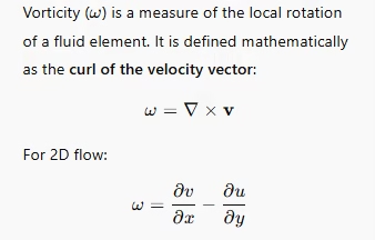
🌊 Physical Meaning:

Positive vorticity = counterclockwise rotation
Negative vorticity = clockwise rotation
Zero vorticity = irrotational flow

🧪 Applications in Civil Engineering:

Enhancing sediment transport predictions in rivers

Identifying vortex regions in dam spillways and around bridge piers

Understanding turbulence near hydraulic structures

② Flow Descriptions

Streamline: A streamline is a curve that is tangent to the velocity vector of the flow at every point. It represents the path a fluid element will follow at a given instant if the flow is steady. No fluid crosses a streamline, making it a useful tool for visualizing the direction of fluid flow. In engineering, streamlines help identify flow separation and recirculation zones, especially around obstacles or in complex geometries.
Pathline: A pathline represents the actual trajectory that a single fluid particle follows over a period of time. Unlike streamlines, which show instantaneous flow direction, pathlines illustrate how a specific fluid element moves as time progresses. Pathlines are especially useful in unsteady flows where fluid particles may follow complex or changing paths. Visualization of pathlines is commonly used in flow experiments using dye or tracer particles.
Streakline: A streakline is the locus of all fluid particles that have passed through a particular fixed point in space. It is the line formed by injecting a continuous stream of dye at a fixed point. This is commonly used in experimental fluid mechanics because it visually shows how fluid has moved through a particular point over time. In steady flow, streaklines, streamlines, and pathlines coincide. However, in unsteady flow, they differ significantly, making streaklines essential for analyzing transient behaviors in flow fields.

In steady flow, all three are identical.

③ Velocity Field

1D: Variation in only one spatial direction, usually along the axis of a pipe or channel. In such cases, the flow properties (such as velocity, pressure, or density) change only along a single axis (typically x-direction), while remaining constant in the other two directions (y and z). For example, in a long, straight pipe with uniform diameter and fully developed laminar flow, velocity varies only along the length of the pipe. This simplification helps in solving governing equations easily using one-dimensional analysis.
2D: In two-dimensional flow, fluid properties such as velocity vary in two spatial directions, typically x and y. This type of flow is common in open channel hydraulics where depth and width vary, such as in canals and rivers. The assumption of negligible variation in the third direction (z-direction) simplifies analysis. Engineers use 2D models to predict surface profiles, flood plains, and sediment transport in civil engineering projects. Computational Fluid Dynamics (CFD) tools also often simulate flows using a 2D approach when symmetry or uniformity in the third dimension can be assumed.
3D: In three-dimensional flow, fluid velocity and other properties vary in all three spatial directions (x, y, and z). This type of flow is the most realistic and complex, representing actual scenarios in nature and engineering. Examples include river currents, atmospheric airflow, and ocean circulation. In civil engineering, 3D flow modeling is essential for:
River and estuary modeling
Bridge pier scour analysis
Wind load analysis on tall structures
Environmental impact studies for pollutant dispersion

To simulate and analyze 3D flow, engineers often rely on advanced Computational Fluid Dynamics (CFD) tools that solve the full Navier-Stokes equations in three dimensions. Although computationally intensive, 3D modeling provides the most accurate representation of real-world fluid behavior, capturing complex features like vortices, secondary flows, and turbulence that cannot be represented in simpler 1D or 2D models.

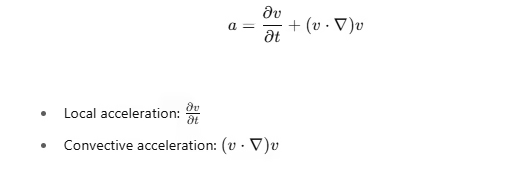
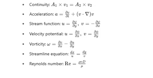
④ Acceleration in Fluids

⑤ Continuity Equation (Incompressible Flow)

⑥ Stream Function (ψ)

⑦ Velocity Potential Function (ϕ)

Used in irrotational flow.

📚 Key Formulas

📄 Conclusion

Fluid Kinematics is an essential part of civil engineering as it provides the foundational understanding of how fluids behave when in motion, particularly in systems where forces are not explicitly considered. It plays a pivotal role in the design and analysis of water supply systems, sewage systems, drainage networks, and irrigation channels. By mastering concepts like streamlines, pathlines, acceleration, and continuity, civil engineers can predict flow behavior, prevent failures in hydraulic structures, and improve the efficiency of fluid transport systems. This understanding also prepares students for more advanced topics like fluid dynamics, sediment transport, and open channel hydraulics, which are vital for real-world engineering applications and competitive exams like JKSSB.